Linear Algebra Basics #

Linear Algebra is a branch of mathematics that deals with vectors, vector spaces and linear transformations. It has wide applications in fields like physics, computer graphics, data analysis and generating yiff.

Vectors #

Vectors are mathematical objects that have both magnitude (size) and direction. They can represent physical quantities like force, velocity or displacement. For example, if you’re a furry running in a park, your velocity is a vector - it has a speed (magnitude) and a direction you’re running in.

This furry has a velocity.

Even this DVD logo has a vector, not just furries, just press the v key and an arrow will display the vector of the logo. Vectors are everywhere, even in your pants! Points are usually denoted with capital letters, like $A$. A directed line segment from $A$ to $B$ is denoted by $\overrightarrow{AB}$.

$$ \vec{v} = \overrightarrow{AB} $$

Vectors are often represented as an array of numbers, where each number corresponds to a coordinate in space. In a 2D plane, a vector $\vec{v}$ can be represented as an ordered pair: $\vec{v} = [v_1, v_2]$. Here $v_1$ and $v_2$ are the components of $\vec{v}$ along the x and y axes respectively. You can also represent it like:

$$ \vec{v} = \begin{bmatrix} v_1 \ v_2 \end{bmatrix} $$

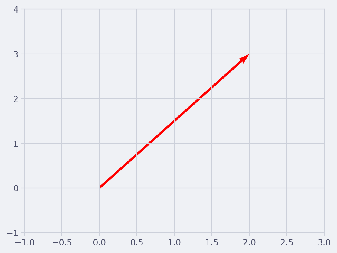
For example, the vector $\vec{v} = [2, 3]$ can be visualized as an arrow starting at the origin $(0, 0)$ and pointing 2 units in the positive x-direction and 3 units in the positive y-direction.

"""
This script creates a 2D vector plot using matplotlib.
It defines a vector 'v' with coordinates (2,3) and plots it on a 2D grid.
The origin of the vector is at (0,0).
"""
import matplotlib.pyplot as plt

# Define the origin
origin = [0], [0]

# Define the vector v
v = [2, 3]

# Create a new figure
plt.figure()

# Plot the vector v
plt.quiver(*origin, *v, color='r', angles='xy', scale_units='xy', scale=1)

# Set the x-limits and y-limits of the plot
plt.xlim(-1, 3)
plt.ylim(-1, 4)

# Add a grid
plt.grid()

# Show the plot
plt.show()

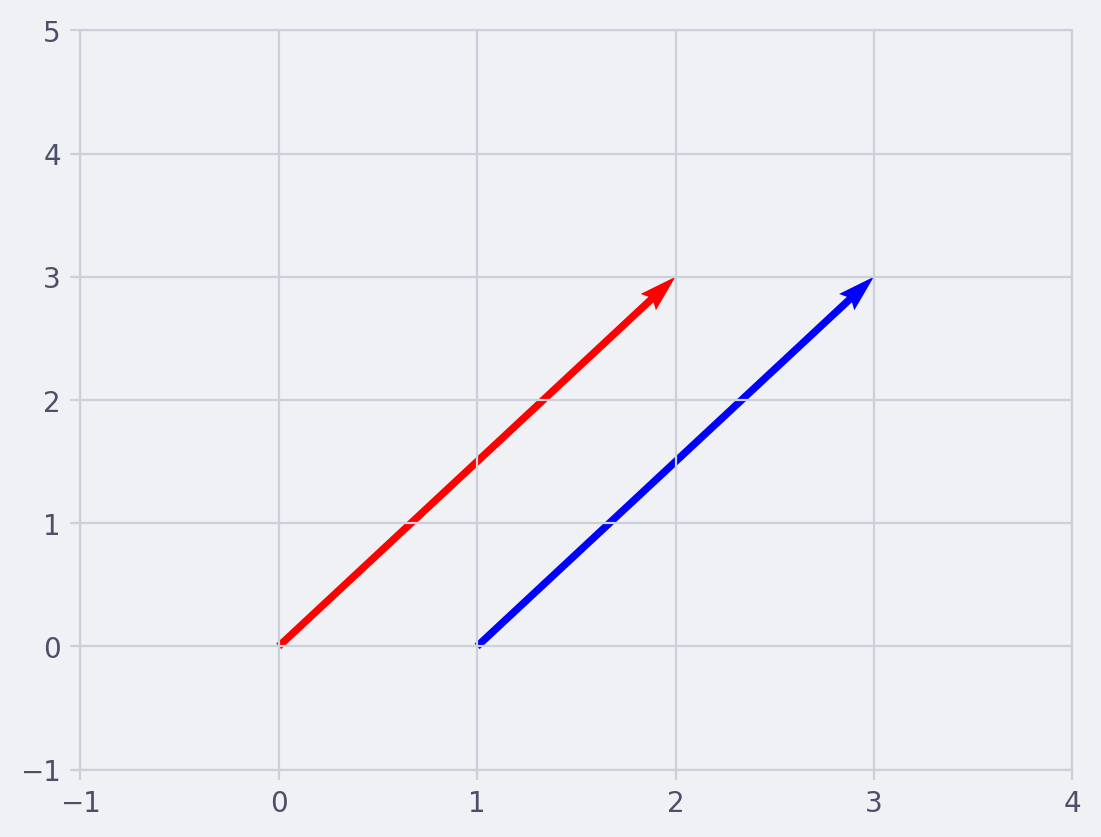
Because we don’t care about the origin of a vector to compare them, only their magnitudes, two parallel vectors that have the same length makes them equal.

$$ \vec{v} = \overrightarrow{AB}, \quad \vec{w} = \overrightarrow{CD} \ \vec{v} = \vec{w} $$

"""
This script plots two vectors, v and w, using matplotlib. The vector v originates
from the origin (0,0), while the vector w starts from a specified point (1,0).
Both vectors are defined as [2, 3], making them parallel to each other.
"""
import matplotlib.pyplot as plt

# Define the origin for v and starting point for w
origin_v = [0], [0]
origin_w = [1], [0]  # Change this to the desired starting point for w

# Define the vectors v and w
v = [2, 3]
w = [2, 3]  # w is parallel to v

# Create a new figure
plt.figure(dpi=200)

# Plot the vector v
plt.quiver(*origin_v, *v, color='r', angles='xy', scale_units='xy', scale=1)

# Plot the vector w
plt.quiver(*origin_w, *w, color='b', angles='xy', scale_units='xy', scale=1)

# Set the x-limits and y-limits of the plot
plt.xlim(-1, 4)
plt.ylim(-1, 5)

# Add a grid
plt.grid()

# Show the plot
plt.show()

Vector Addition #

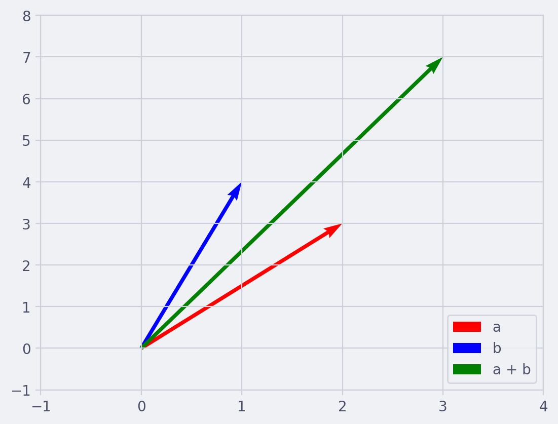
If you have two vectors, you can add them together to get a new vector. This is done by adding the corresponding components of the vectors. For example if $\vec{a} = [2, 3]$ and $\vec{b} = [1, 4]$ then $\vec{a} + \vec{b} = [2+1, 3+4] = [3, 7]$.

"""
This script visualizes the addition of two vectors using matplotlib.

It first defines two 2D vectors 'a' and 'b', then calculates their sum 'c'.
The vectors are then plotted on a 2D grid using matplotlib's quiver function.
"""
import matplotlib.pyplot as plt
import numpy as np

# Define the vectors
a = np.array([2, 3])
b = np.array([1, 4])

# Calculate the sum of the vectors
c = a + b

# Create a new figure
plt.figure(dpi=200)

# Plot the vectors a, b, and c
plt.quiver(0, 0, a[0], a[1], angles='xy', scale_units='xy', scale=1, color='r', label='a')
plt.quiver(0, 0, b[0], b[1], angles='xy', scale_units='xy', scale=1, color='b', label='b')
plt.quiver(0, 0, c[0], c[1], angles='xy', scale_units='xy', scale=1, color='g', label='a + b')

# Set the x-limits and y-limits of the plot
plt.xlim(-1, 4)
plt.ylim(-1, 8)

# Add a grid
plt.grid()

# Add a legend
plt.legend(loc="lower right")

# Show the plot
plt.show()

Scalar Multiplication #

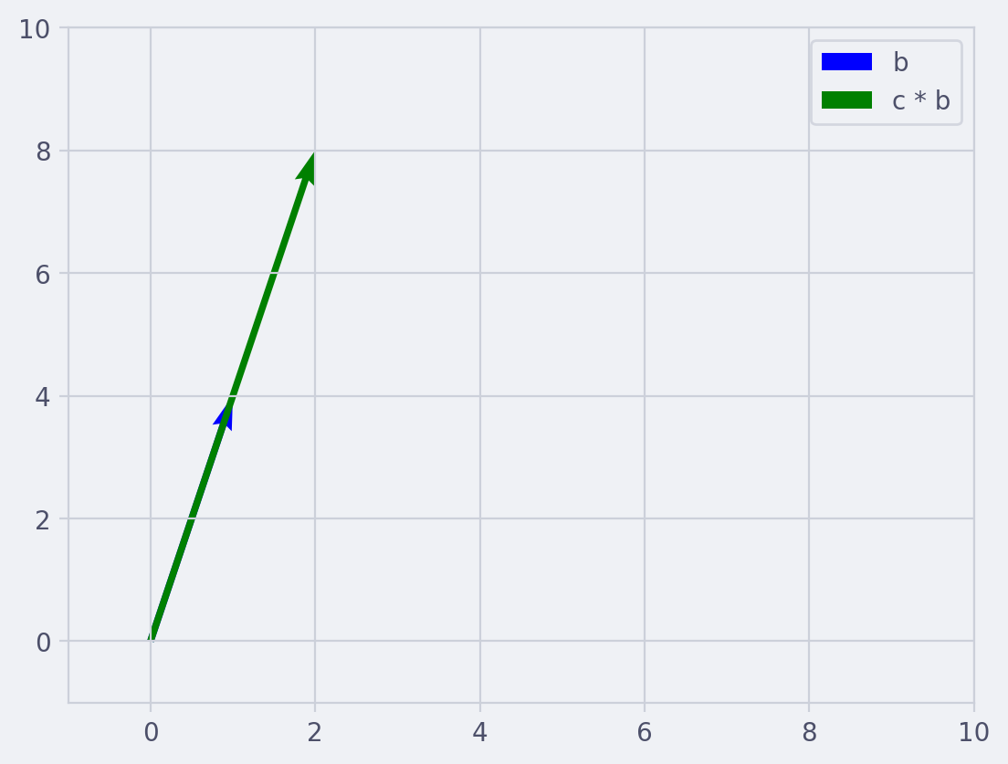
You can multiply a vector by a scalar (regular number) to get a new vector. This is done by multiplying each component of the vector by the scalar. For example if $c = 2$ and $\vec{b} = [1,4]$ then $c * \vec{b} = [23, 24] = [6, 8]$.

"""
This script demonstrates the scalar multiplication of a vector.
It defines a vector 'b' and a scalar 'c', calculates the scalar multiplication
of the vector, and then plots the original vector and the result of the scalar
multiplication on a 2D grid. The vectors are represented as arrows originating
from the origin (0,0).
"""
import matplotlib.pyplot as plt
import numpy as np

# Define the vector and scalar
b = np.array([1, 4])
c = 2

# Calculate the scalar multiplication of the vector
d = c * b

# Create a new figure
plt.figure(dpi=200)

# Plot the vectors b and d
plt.quiver(0, 0, b[0], b[1], angles='xy', scale_units='xy', scale=1, color='b', label='b')
plt.quiver(0, 0, d[0], d[1], angles='xy', scale_units='xy', scale=1, color='g', label='c * b')

# Set the x-limits and y-limits of the plot
plt.xlim(-1, 10)
plt.ylim(-1, 10)

# Add a grid
plt.grid()

# Add a legend
plt.legend()

# Show the plot
plt.show()

Dot Product #

The dot product of two vectors is a scalar quantity that is the sum of the products of the corresponding components of the vectors. For example if $\vec{e} = [2, 3]$ and $\vec{f} = [4, 5]$, then $\vec{e} \cdot \vec{f} = 24 + 35 = 23$

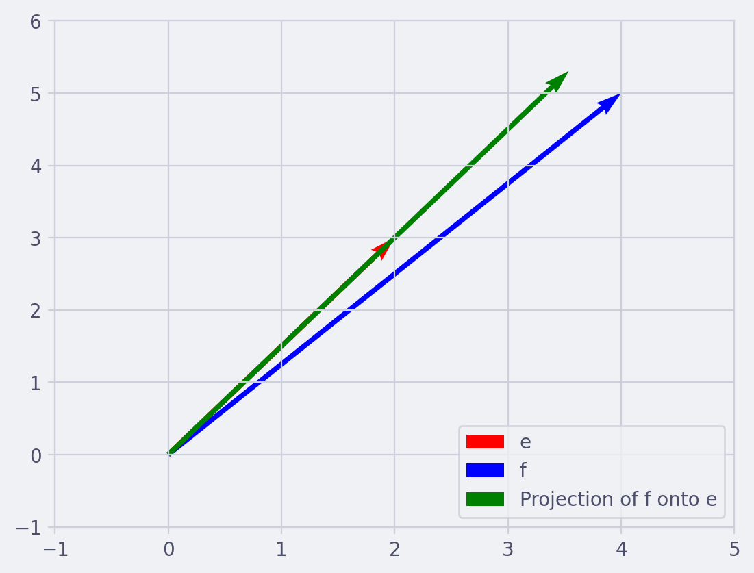
This is a geometric interpretation of the dot product, and it’s particularly useful when thinking about the dot product as a measure of the similarity between two vectors: if $\vec{f}$ is very similar to $\vec{e}$ (i.e., it points in the same direction), then its projection onto $\vec{e}$ will be long, and so the dot product will be large. Conversely, if $\vec{f}$ is dissimilar to $\vec{e}$ (i.e., it points in a very different direction), then its projection onto $\vec{e}$ will be short, and so the dot product will be small.

The magnitude of the cross product vector equals the area of the parallelogram formed by the two original vectors.

"""
This script calculates and visualizes the dot product and projection of two vectors.

The script first defines two vectors, e and f. It then calculates the dot product of
these vectors and the projection of vector f onto vector e. The vectors, their dot
product, and the projection are then plotted on a 2D grid using matplotlib.
Finally, the script prints the calculated dot product.
"""
import matplotlib.pyplot as plt
import numpy as np

# Define the vectors
e = np.array([2, 3])
f = np.array([4, 5])

# Calculate the dot product of the vectors
g = np.dot(e, f)

# Calculate the projection of f onto e
proj = (np.dot(e, f) / np.linalg.norm(e)**2) * e

# Create a new figure
plt.figure(dpi=200)

# Plot the vectors e and f
plt.quiver(0, 0, e[0], e[1], angles='xy', scale_units='xy', scale=1, color='r', label='e')
plt.quiver(0, 0, f[0], f[1], angles='xy', scale_units='xy', scale=1, color='b', label='f')

# Plot the projection of f onto e
plt.quiver(0, 0, proj[0], proj[1], angles='xy', scale_units='xy', scale=1, color='g', label='Projection of f onto e')

# Set the x-limits and y-limits of the plot
plt.xlim(-1, 5)
plt.ylim(-1, 6)

# Add a grid
plt.grid()

# Add a legend
plt.legend(loc="lower right")

# Show the plot
plt.show()

# Print the dot product
print("The dot product of vectors e and f is: ", g)

Magnitude (or Length) #

The magnitude of a vector $\vec{g} = [a, b]$ is given by the square root of the sum of the squares of its components. This is denoted as $||\vec{g}||$ and calculated as $||\vec{g}|| = \sqrt{a^2 + b^2}$

import numpy as np

def calculate_magnitude(vector):
    """
    Calculate the magnitude of a vector.

    The magnitude of a vector is the length of the vector in n-dimensional space,
    computed as the square root of the sum of the absolute squares of its components.

    Parameters:
    vector : numpy.ndarray
        A numpy array representing the vector.

    Returns:
    float: The magnitude of the vector.
    """
    magnitude = np.linalg.norm(vector)
    return magnitude

# Example usage:
g = np.array([3, 4])
print("The magnitude of the vector g is:", calculate_magnitude(g))

Matrices #

A matrix is a rectangular array of numbers arranged in rows and columns. Matrices are used to represent and manipulate linear transformations, which are functions that map vectors to vectors while preserving vector addition and scalar multiplication. Each number in the matrix is called an element or entry. The position of an element is defined by its row number and column number.

A $2 \times 2$ matrix can be represented as follows:

$$A = \begin{bmatrix} a & b \ c & d \end{bmatrix}$$

Matrix Addition and Subtraction #

Matrices can be added or subtracted element by element if they are of the same size. For example if we have two $2 \times 2$ matrices $A$ and $B$ then the sum $A+B$ is a new $2 \times 2$ matrix where each element is the sum of the corresponding elements in $A$ and $B$.

It can be represented as:

$$ A + B = \begin{bmatrix} a1 & b1 \ c1 & d1 \end{bmatrix} + \begin{bmatrix} a2 & b2 \ c2 & d2 \end{bmatrix} = \begin{bmatrix} a1+a2 & b1+b2 \ c1+c2 & d1+d2 \end{bmatrix} $$

This is how you can create a $2 \times 2$ matrix with numpy:

import numpy as np

# Create a 2x2 matrix
A = np.array([[1, 2], [3, 4]])

If we have two matrices $A$ and $B$ of the same size representing linear transformations, their sum $A + B$ also represents a linear transformation. The sum transformation $(A + B)$ applied to any vector $\vec{v}$ is equal to $A(\vec{v}) + B(\vec{v})$. This property is known as linear separability.

$$ (A + B)(\vec{v}) = A(\vec{v}) + B(\vec{v}) $$

Scalar Multiplication of a Matrix #

A matrix can be multiplied by a scalar. This is done by multiplying each element of the matrix by the scalar.

$$kA = k \cdot \begin{bmatrix} a & b \ c & d \end{bmatrix} = \begin{bmatrix} ka & kb \ kc & kd \end{bmatrix}$$

Matrix Multiplication #

The multiplication of two matrices is more complex than their addition. For two matrices to be multiplied, the number of columns in the first matrix must be equal to the number of rows in the second matrix.

$$AB = \begin{bmatrix} a1 & b1 \ c1 & d1 \end{bmatrix} \cdot \begin{bmatrix} a2 & b2 \ c2 & d2 \end{bmatrix} = \begin{bmatrix} a1a2 + b1c2 & a1b2 + b1d2 \ c1a2 + d1c2 & c1b2 + d1d2 \end{bmatrix}$$

Matrix multiplication corresponds to function composition of linear transformations. If $A$ and $B$ are matrices representing linear transformations, then $AB$ represents the transformation that first applies $B$ and then applies $A$.

For two matrices to be multiplied, the number of columns in the first matrix must equal the number of rows in the second matrix.

Identity Matrix #

This is a special type of square matrix where all the elements of the principal diagonal (from the upper left to the bottom right) are ones and all other elements are zeros. The identity matrix play a similar role in matrix algebra as the number 1 in regular algebra. Here are some example ones:

$$ I_2 = \begin{bmatrix} 1 & 0 \ 0 & 1 \end{bmatrix} \quad I_3 = \begin{bmatrix} 1 & 0 & 0 \ 0 & 1 & 0 \ 0 & 0 & 1 \end{bmatrix} \quad I_4 = \begin{bmatrix} 1 & 0 & 0 & 0 \ 0 & 1 & 0 & 0 \ 0 & 0 & 1 & 0 \ 0 & 0 & 0 & 1 \end{bmatrix} $$

The identity matrix plays a similar role in matrix operations as the number 1 does in real number operations. When you multiply any square matrix by the identity matrix of the same order, you get the original matrix back, regardless of the order of multiplication. This is expressed as:

$$ A \cdot I = I \cdot A = A $$

• Where $A$ is any square matrix,
• $I$ is the identity matrix of the same order as $A$.

Determinant #

The determinant is a special number that can be calculated from a square matrix. It has many important properties and uses, such as providing the solution of a system of linear equations.

$$det(A) = det\begin{bmatrix} a & b \ c & d \end{bmatrix} = ad - bc$$

Inverse #

The inverse of a matrix $A$ is another matrix, denoted as $A^{-1}$, such that when $A$ is multiplied by $A^{-1}$, the result is the identity matrix. Not all matrices have an inverse.

$$A^{-1} = \frac{1}{det(A)} \begin{bmatrix} d & -b \ -c & a \end{bmatrix}$$

Transpose #

The transpose of a matrix is a new matrix whose rows are the columns of the original matrix and whose columns are the rows.

$$A^T = \begin{bmatrix} a & c \ b & d \end{bmatrix}$$

Eigenvalues and Eigenvectors #

Eigenvalues #

An eigenvalue of a square matrix $A$ is a scalar $\lambda$ that satisfies the equation:

$$ A\vec{v} = \lambda\vec{v} $$

Where $\vec{v}$ is a non-zero vector. This equation can be rearranged as:

$$ (A - \lambda I)\vec{v} = \vec{0} $$

Where $I$ is the identity matrix of the same size as $A$, and $\vec{0}$ is the zero vector. The scalars $\lambda$ that satisfy this equation are the eigenvalues of $A$.

To find the eigenvalues of a matrix, we set the determinant of $(A - \lambda I)$ equal to zero and solve for $\lambda$:

$$ \det(A - \lambda I) = 0 $$

This equation is known as the characteristic equation of $A$, and its solutions are the eigenvalues of $A$.

Here’s an example in Python using NumPy to find the eigenvalues of a $3 \times 3$ matrix:

import numpy as np

# Define the matrix A
A = np.array([[1, 2, 3],
              [4, 5, 6],
              [7, 8, 9]])

# Calculate the eigenvalues
eigenvalues, _ = np.linalg.eig(A)
print("Eigenvalues: ", eigenvalues)

The script uses the np.linalg.eig function to calculate the eigenvalues of the matrix A. This function returns a tuple consisting of a vector (the eigenvalues of A) and an array (the corresponding eigenvectors of A). In this case, the script only keeps the eigenvalues and ignores the eigenvectors by storing them in _.

Eigenvectors #

An eigenvector of a matrix $A$ is a non-zero vector $\vec{v}$ that satisfies the equation:

$$ A\vec{v} = \lambda\vec{v} $$

Where $\lambda$ is an eigenvalue of $A$ corresponding to $\vec{v}$. For each eigenvalue $\lambda$, there may be one or more eigenvectors associated with it.

To find the eigenvectors corresponding to an eigenvalue $\lambda$, we substitute $\lambda$ into the equation $(A - \lambda I)\vec{v} = \vec{0}$ and solve for $\vec{v}$.

Here’s an example in Python using NumPy to find the eigenvectors of a $2 \times 2$ matrix:

import numpy as np

# Define the matrix A
A = np.array([[2, 1],
              [1, 3]])

# Calculate the eigenvalues and eigenvectors
eigenvalues, eigenvectors = np.linalg.eig(A)

print("Eigenvalues: ", eigenvalues)

# Print the eigenvectors
for i in range(len(eigenvalues)):
    print(f"Eigenvector for eigenvalue {eigenvalues[i]}: {eigenvectors[:, i]}")

In this example, we first calculate the eigenvalues and eigenvectors of the matrix A using np.linalg.eig. The function returns the eigenvalues as a 1D array, and the eigenvectors as a 2D array, where each column corresponds to an eigenvector associated with the eigenvalue at the same index.

We then iterate over the eigenvalues and print the corresponding eigenvectors. Note that the eigenvectors are normalized to have a length of 1.

Eigenvectors have many important properties and applications. For example, they can be used to diagonalize a matrix, which simplifies many matrix computations. They are also useful in fields like quantum mechanics, where they represent the possible states of a system.

Properties of Eigenvalues and Eigenvectors #

Some important properties of eigenvalues and eigenvectors include:

Linearity: If $\vec{v}_1$ and $\vec{v}_2$ are eigenvectors of $A$ with corresponding eigenvalues $\lambda_1$ and $\lambda_2$, then any linear combination $c_1\vec{v}_1 + c_2\vec{v}_2$ is also an eigenvector of $A$ with the same eigenvalue $c_1\lambda_1 + c_2\lambda_2$.

Diagonalizability: If a square matrix $A$ has $n$ linearly independent eigenvectors, then $A$ is diagonalizable. This means that there exists an invertible matrix $P$ such that $P^{-1}AP$ is a diagonal matrix, where the diagonal entries are the eigenvalues of $A$.

Geometric Multiplicity and Algebraic Multiplicity: The geometric multiplicity of an eigenvalue $\lambda$ is the dimension of the corresponding eigenspace (the space spanned by the eigenvectors associated with $\lambda$). The algebraic multiplicity of $\lambda$ is the multiplicity of $\lambda$ as a root of the characteristic equation $\det(A - \lambda I) = 0$. The algebraic multiplicity is always greater than or equal to the geometric multiplicity.

Orthogonality of Eigenvectors: If $A$ is a real symmetric matrix (or a complex hermitian matrix), then the eigenvectors corresponding to distinct eigenvalues are orthogonal to each other.