Orthogonal Matrices #

An orthogonal matrix is a square matrix whose rows and columns are orthogonal unit vectors. In other words, it is a matrix whose columns (and rows) form an orthonormal basis for the vector space they span, meaning they are mutually perpendicular unit vectors.

More precisely, a matrix $Q$ is orthogonal if it satisfies the following condition:

$$ Q^T Q = Q Q^T = I $$

Where $Q^T$ is the transpose of $Q$, and $I$ is the identity matrix of the same dimensions.

This property implies that orthogonal matrices are invertible, and their inverse is simply their transpose.

$$ Q = \begin{bmatrix} 1 & 0 \ 0 & 1 \end{bmatrix} $$

This matrix represents the identity matrix in two-dimensional space. This matrix is significant because it serves as the multiplicative identity in linear algebra, meaning any vector multiplied by this matrix will remain unchanged.

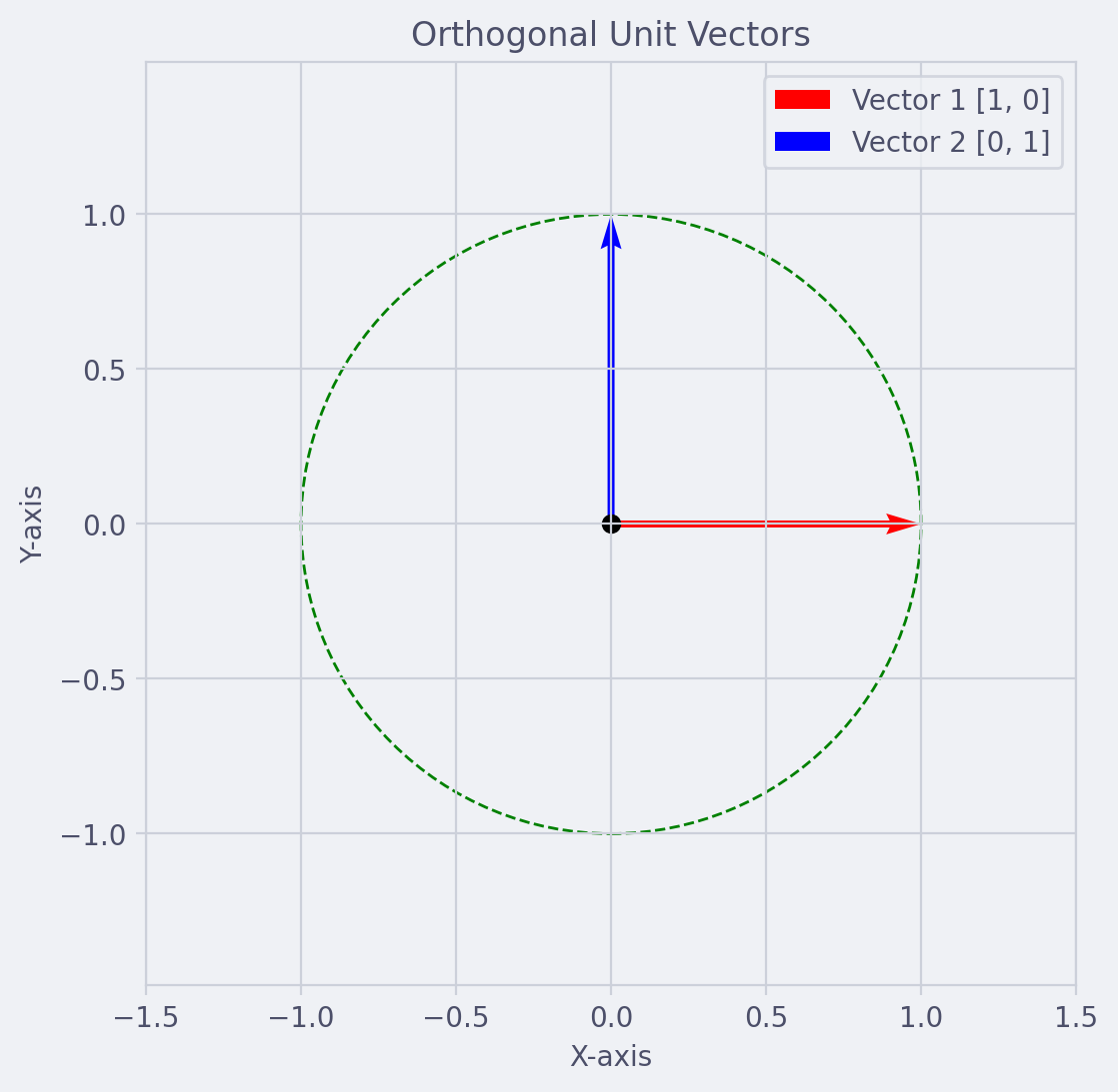
The accompanying diagram illustrates two orthogonal unit vectors in a two-dimensional coordinate system. These vectors are represented as arrows originating from the origin $(0,0)$ and extending to the points $(1,0)$ and $(0,1)$, respectively.

Both vectors have a magnitude of 1, which positions them on the unit circle—a green dashed circle with a radius of 1 that encompasses both vectors. The unit circle is a fundamental concept in trigonometry and complex analysis, as it represents all possible angles and their corresponding points in the Cartesian plane.

The Inverse of an Orthogonal Matrix #

One of the properties of an orthogonal matrix is that its inverse is equal to its transpose:

$$ Q^{-1} = Q^T $$

This means that to find the inverse of an orthogonal matrix, one simply needs to transpose the matrix—switch the rows and columns.

Consider the following orthogonal matrix:

$$ Q = \begin{bmatrix} \cos(\theta) & -\sin(\theta) \ \sin(\theta) & \cos(\theta) \end{bmatrix} $$

The inverse of this matrix, which represents a rotation by angle $\theta$, is given by:

$$ Q^{-1} = Q^T = \begin{bmatrix} \cos(\theta) & \sin(\theta) \ -\sin(\theta) & \cos(\theta) \end{bmatrix} $$

This inverse matrix represents a rotation in the opposite direction, effectively undoing the original rotation.

Preserving Vector Norms #

When an orthogonal matrix multiplies a vector, the length (or norm) of the vector is preserved. This is why orthogonal transformations are also called isometries. Mathematically, for any vector $\vec{v}$, we have:

$$ ||Q\vec{v}|| = ||\vec{v}|| $$

Determinant of Orthogonal Matrices #

The determinant of an orthogonal matrix is always either +1 or -1. This is a direct consequence of the matrix being a product of reflections and rotations, both of which preserve the area (in 2D) or volume (in 3D) up to a sign. Thus:

$$ \text{det}(Q) = \pm 1 $$

Eigenvalues and Eigenvectors #

The eigenvalues of an orthogonal matrix are always of absolute value 1. They can be either real ($\pm 1$) or complex numbers with a magnitude of 1. This reflects the fact that orthogonal matrices correspond to rotations and reflections, which do not change the magnitude of vectors. For an orthogonal matrix, the eigenvalues are values that satisfy the equation:

$$ Q\vec{v} = \lambda \vec{v} $$

where $\vec{v}$ is a non-zero vector (eigenvector), and $\lambda$ is a scalar (eigenvalue). Since orthogonal matrices represent rotations and reflections, their eigenvalues are of absolute value 1, which means they lie on the unit circle in the complex plane.

Consider the orthogonal matrix representing a rotation by angle $\theta$:

$$ Q = \begin{bmatrix} \cos(\theta) & -\sin(\theta) \ \sin(\theta) & \cos(\theta) \end{bmatrix} $$

The eigenvalues of this matrix are complex numbers $e^{i\theta}$ and $e^{-i\theta}$, which correspond to rotations by $\theta$ and $-\theta$ respectively. The eigenvectors associated with these eigenvalues are also complex and represent the directions that are invariant under the rotation.

In physical terms, the eigenvectors of an orthogonal matrix represent the axes of rotation or reflection, and the eigenvalues describe the nature of the transformation along those axes. For instance, an eigenvalue of +1 indicates that the vector remains unchanged, while -1 indicates a reflection.

Application in Complex Systems #

Orthogonal matrices play a crucial role in simplifying complex systems. For instance, in the diagonalization of a matrix, orthogonal matrices can be used to transform a matrix into a diagonal form, which is much easier to analyze and work with.

Example #1 #

"""
This script demonstrates the properties of orthogonal matrices in linear algebra using a 3x3 matrix.

It defines a 3x3 orthogonal matrix 'Q', calculates its transpose 'Q_T' and its inverse 'Q_inv'.
It then checks if the transpose is equal to the inverse, which is the defining property of an orthogonal matrix.
If 'Q' is orthogonal, it prints 'Q is orthogonal: True', otherwise it prints 'Q is orthogonal: False'.

Note: This script uses the numpy library for matrix operations.
"""
import numpy as np

# Define a 3x3 orthogonal matrix
Q = np.array([[0, 0, 1],
              [1, 0, 0],
              [0, 1, 0]])

# Calculate its transpose
Q_T = Q.T

# Calculate its inverse
Q_inv = np.linalg.inv(Q)

# Check if the transpose is equal to the inverse
print("Q is orthogonal:", np.allclose(Q_T, Q_inv))

Example #2 #

This script generates and checks orthogonal matrices.

import numpy as np
import matplotlib.pyplot as plt

def generate_orthogonal(n):
    """
    Generate a random n x n orthogonal matrix.
    """
    H = np.random.randn(n, n)
    Q, R = np.linalg.qr(H)
    return Q

def is_orthogonal(Q):
    """
    Check if a matrix is orthogonal.
    """
    return np.allclose(Q.T, np.linalg.inv(Q))

# Generate and check 20 orthogonal matrices
for i in range(1, 21):
    Q = generate_orthogonal(3)
    print(f"Matrix {i} is orthogonal: {is_orthogonal(Q)}")

    # Plot the matrix
    plt.figure(figsize=(6, 6))
    plt.imshow(Q, cmap='viridis')
    plt.title(f"Orthogonal Matrix {i}")
    plt.colorbar()
    plt.show()

1. The script first defines the generate_orthogonal(n) function which generates a random $n \times n$ orthogonal matrix. It first creates a random $n \times n$ matrix H using np.random.randn(n, n). Then, it uses the QR decomposition function np.linalg.qr(H) to decompose this matrix into Q (an orthogonal matrix) and R (an upper triangular matrix). The function returns Q.
2. Then it defines the is_orthogonal(Q) function which checks if a matrix Q is orthogonal. It does this by comparing the transpose of Q (denoted Q.T) with the inverse of Q (denoted np.linalg.inv(Q)). If Q is orthogonal, these two matrices will be close to each other (within a certain tolerance), so np.allclose(Q.T, np.linalg.inv(Q)) will return True.
3. The script then generates and checks 20 orthogonal matrices. For each matrix, it uses generate_orthogonal(3) to generate a $3 \times 3$ orthogonal matrix, checks if the matrix is orthogonal using is_orthogonal(Q), and prints the result. It also plots the matrix using matplotlib.